幂律分布 - Power Law Distribution

---

参考:

• Veritasium - This graph will change how you see the world

---

掷硬币游戏：三种分布的生成机制

正态分布 (Normal Distribution)

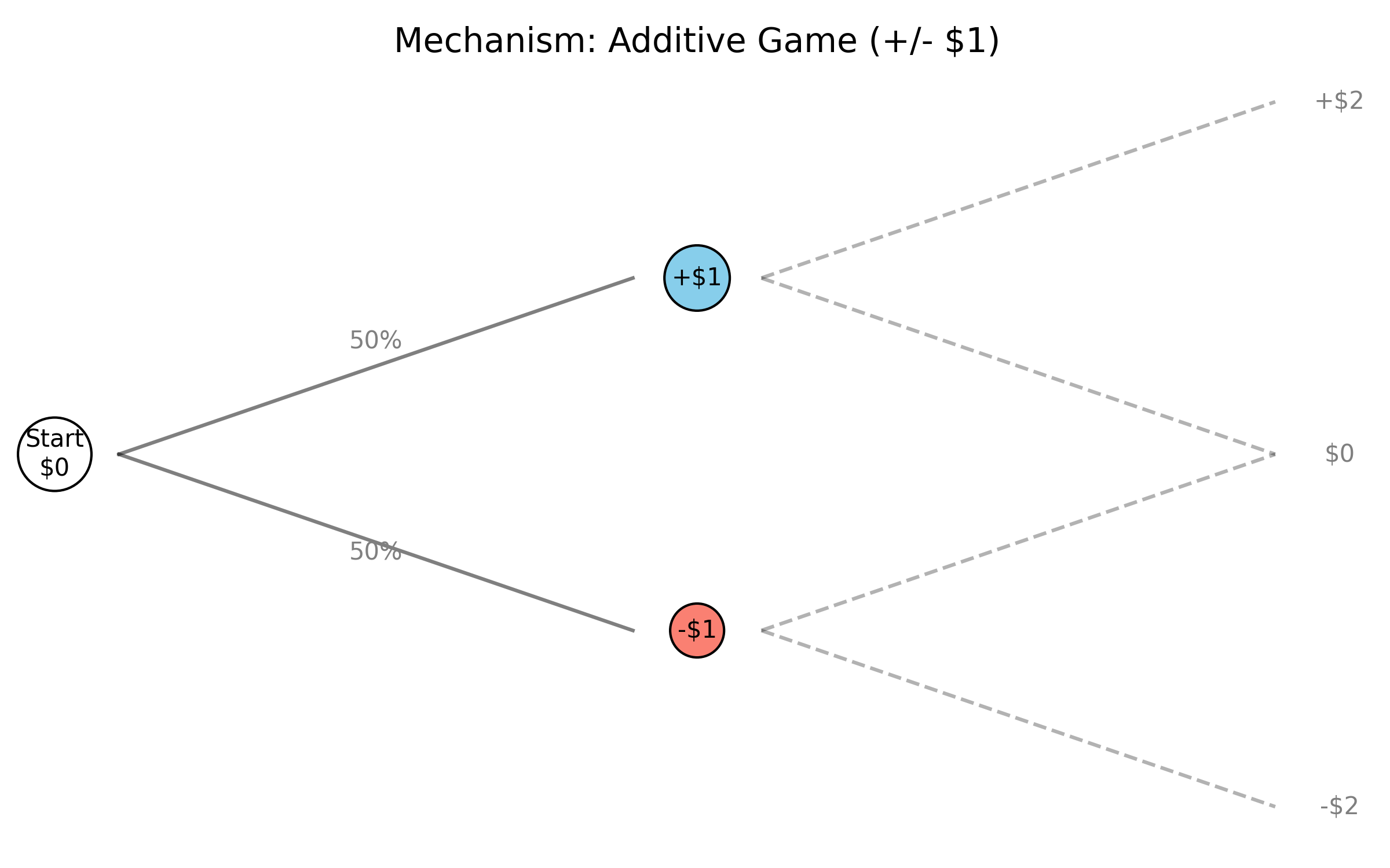
• 生成机制：相加过程
  • 当一个系统受到大量相互独立的随机因素影响，且这些因素是相加关系时，结果趋向于正态分布。
  • 例子：每次掷硬币正面收益$1，反面损失$1。连续多次后的总财富分布。
• 数学性质：
  • 典型尺度：数据围绕一个明确的平均值（Average）聚集。
  • 薄尾 (Thin Tail)：极端异常值（Outliers）几乎不可能发生（例如不可能有人身高是平均值的5倍）。
  • 中心极限定理 (CLT) 的体现。

对数正态分布 (Lognormal Distribution)

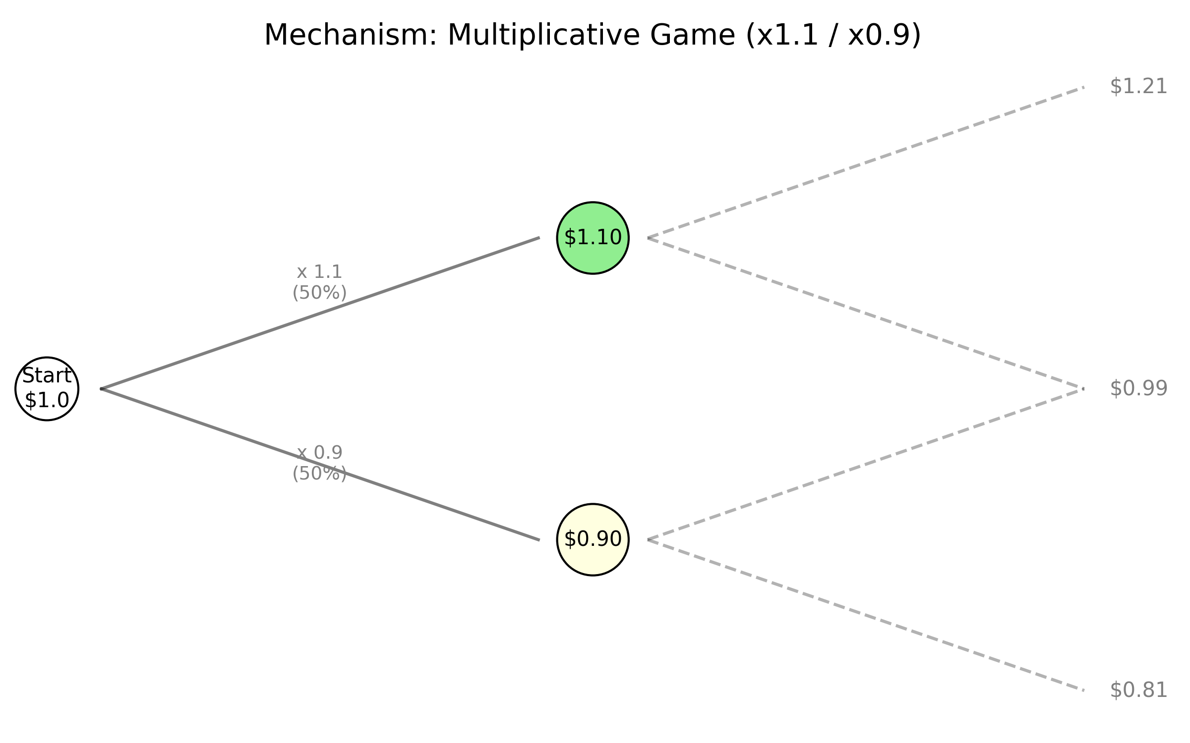
• 生成机制：相乘过程
  • 当随机效应是相乘而非相加时产生。
  • 例子：初始资金 $1，每次掷硬币正面乘以 1.1，反面乘以 0.9。连续多次后的总财富分布。
  • 数学逻辑：根据对数性质 $\log(a \cdot b) = \log(a) + \log(b)$，乘积的对数变成了和，因此数据的对数服从正态分布。
• 数学性质：
  • 偏态 (Skewed)：分布不对称，长尾在右侧。会产生贫富差距，但不如幂律分布极端。

幂律分布 (Power Law Distribution)

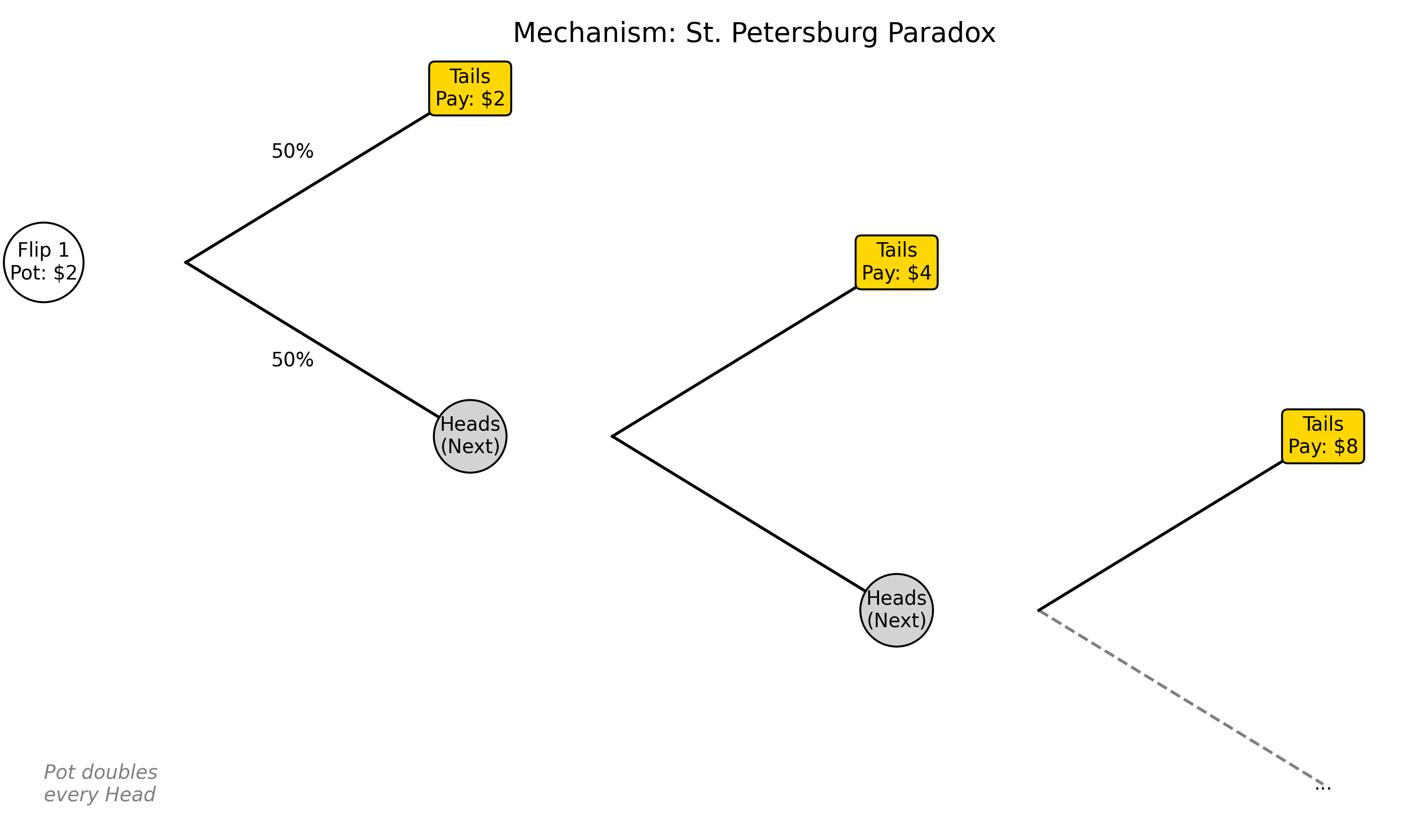
• 生成机制：
  1. 圣彼得堡悖论：不断抛硬币，直到首次出现正面为止，若第 $n$ 次才首次出现正面，则奖金为 $2^n$ 元；
  2. 自组织临界性 (Self-Organized Criticality, SOC)：系统自然演化到临界点（Critical Point），此时系统没有特征尺度，任何微小的扰动都可能引发任意规模的雪崩。
  3. 优先连接：Barabási–Albert模型（互联网链接模型）。新节点更倾向于连接到已有很多连接的节点。
• 数学性质：
  • 无标度 (Scale-free)：系统没有固定的特征尺度（$?$阶矩，取决于幂指数）。
  • 肥尾 (Fat/Heavy Tail)：极端事件（黑天鹅）发生的概率远高于正态分布的预期。
  • 分形 (Fractal)：具有自相似性，在不同尺度下观察到的结构模式相同。
  • 双对数线性：在 Log-Log 图上表现为一条斜率为负的直线，公式为 $P(x) \propto x^{-\alpha}$。

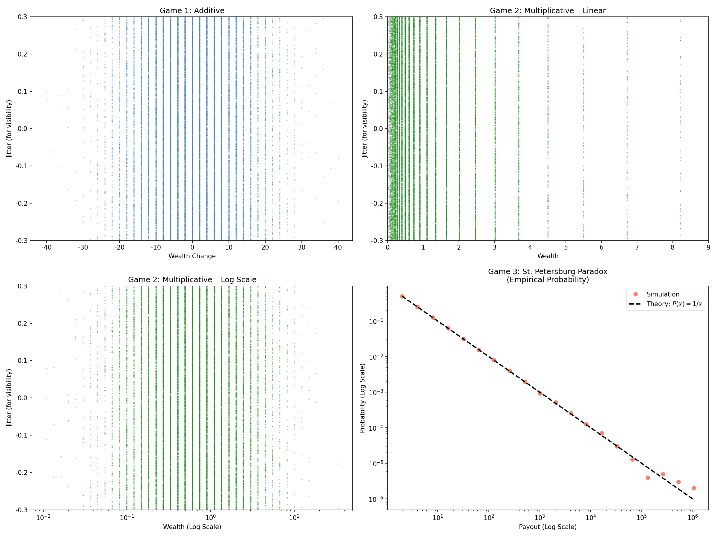
模拟

代码

import matplotlib.pyplot as plt
import numpy as np

# Set generic font to avoid issues
plt.rcParams['font.sans-serif'] = ['DejaVu Sans']
plt.rcParams['axes.unicode_minus'] = False

def run_simulations_and_plot():
    N_TRIALS = int(1e6)
    N_FLIPS = 100

    # --- Simulate ---
    # Game 1: Additive
    flips1 = np.where(np.random.randint(0, 2, (N_TRIALS, N_FLIPS)) == 0, -1, 1)
    results1 = np.sum(flips1, axis=1)

    # Game 2: Multiplicative
    flips2 = np.where(np.random.randint(0, 2, (N_TRIALS, N_FLIPS)) == 0, 0.9, 1.1)
    results2 = np.prod(flips2, axis=1)

    # Game 3: St. Petersburg
    k = np.random.geometric(p=0.5, size=N_TRIALS)
    results3 = 2.0 ** k

    # --- For visualization, take a manageable sample to avoid overplotting ---
    SAMPLE_SIZE = int(2e4)
    idx = np.random.choice(N_TRIALS, size=SAMPLE_SIZE, replace=False)
    sample1 = results1[idx]
    sample2 = results2[idx]

    # Add jitter on y-axis
    jitter = np.random.uniform(-0.3, 0.3, size=SAMPLE_SIZE)

    # --- Plotting ---
    fig, axes = plt.subplots(2, 2, figsize=(16, 12))

    # Game 1: Additive (Scatter with jitter)
    axes[0, 0].scatter(sample1, jitter, s=1, alpha=0.3, color='steelblue')
    axes[0, 0].set_title('Game 1: Additive', fontsize=12)
    axes[0, 0].set_xlabel('Wealth Change')
    axes[0, 0].set_ylabel('Jitter (for visibility)')
    axes[0, 0].set_ylim(-0.3, 0.3)

    # Game 2: Multiplicative – Linear scale
    axes[0, 1].scatter(sample2, jitter, s=1, alpha=0.3, color='forestgreen')
    axes[0, 1].set_title('Game 2: Multiplicative – Linear', fontsize=12)
    axes[0, 1].set_xlabel('Wealth')
    axes[0, 1].set_ylabel('Jitter (for visibility)')
    axes[0, 1].set_xlim(0, 9)
    axes[0, 1].set_ylim(-0.3, 0.3)

    # Game 2: Multiplicative – Log scale (x-axis only)
    axes[1, 0].scatter(sample2, jitter, s=1, alpha=0.3, color='forestgreen')
    axes[1, 0].set_xscale('log')
    axes[1, 0].set_title('Game 2: Multiplicative – Log Scale', fontsize=12)
    axes[1, 0].set_xlabel('Wealth (Log Scale)')
    axes[1, 0].set_ylabel('Jitter (for visibility)')
    axes[1, 0].set_ylim(-0.3, 0.3)

    # Game 3: St. Petersburg
    unique_payouts, counts = np.unique(results3, return_counts=True)
    probabilities = counts / N_TRIALS
    sort_idx = np.argsort(unique_payouts)
    unique_payouts = unique_payouts[sort_idx]
    probabilities = probabilities[sort_idx]
    axes[1, 1].loglog(unique_payouts, probabilities, 'o', color='salmon', markersize=6, label='Simulation')

    x_theory = unique_payouts
    y_theory = 1.0 / x_theory
    axes[1, 1].loglog(x_theory, y_theory, 'k--', linewidth=2, label=r'Theory: $P(x) = 1/x$')

    axes[1, 1].set_title('Game 3: St. Petersburg Paradox\n(Empirical Probability)', fontsize=12)
    axes[1, 1].set_xlabel('Payout (Log Scale)')
    axes[1, 1].set_ylabel('Probability (Log Scale)')
    axes[1, 1].legend()

    plt.tight_layout()
    plt.savefig("simulation_results_scatter_jitter.png", dpi=150)
    print("Saved simulation_results_scatter_jitter.png")

if __name__ == "__main__":
    run_simulations_and_plot()

运行结果

例子

物理学与地质学

• 森林火灾：火灾覆盖面积服从幂律。人工可控的计划烧除有助于抑制极端大规模火灾的发生。
• 相变：磁性材料中的原子磁矩倾向于与邻近原子平行排列（降低能量）形成磁畴。但热扰动倾向于使其随机化。加热到居里温度时，系统进入临界区域，长程序逐渐消失，自旋涨落的关联长度散。在临界点，磁化涨落呈现出标度不变性，不同尺度的磁化团簇共存，其尺寸分布服从幂律，这是连续相变的典型特征。
• 沙堆模型（Bak-Tang-Wiesenfeld 模型）：沙粒崩塌的规模分布。真实的沙子不符合。
• 地震：小地震极多，大地震极少。Gutenberg-Richter Law: 释放能量与发生频率呈幂律关系。

经济学与社会学

• 帕累托法则 (Pareto Principle)：财富分布。帕累托发现意大利、英国等国的收入分布，双对数下斜率约为 -1.5。
• 战争：战争造成的死亡人数分布。
• 金融市场：股票市场崩盘的规模、风险投资的回报（极少数初创公司带来绝大部分回报）。
• 互联网：网页的链接数量（如 Yahoo/Google 连接数巨大，大多数网站连接数极少）、YouTube 视频播放量。
• 学术引用：知名学者/机构更易获得关注；高被引论文更可能被新论文引用。
• Zipf 定律：在自然语言中，单词的频率$f$与其排名$r$成反比。

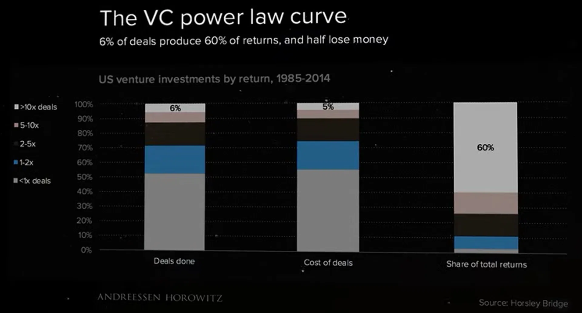
• 投资数量
  • 一半的投资项目都会赔钱。
  • 成功仅占 6%。
• 投资成本
  • 风投家花在失败项目上的钱，和花在成功项目上的钱比例差不多。这意味着在事前，没人能精准预测谁是那个 6%。
• 总回报份额
  • 仅 6% 的顶级项目创造了 60% 的总回报。
  • 占了一半数量的失败项目对回报的贡献几乎为零。

生物学与生态学

• 物种分布、物种灭绝规模、代谢率。

幂律分布的矩收敛条件

对于幂律分布 $p(x) = C x^{-\alpha}$ (定义在 $x \geq x_{min}$)，其 $m$ 阶矩（Moment）定义为：

\[E[X^m] = \int_{x_{min}}^{\infty} x^m \cdot C x^{-\alpha} dx = C \int_{x_{min}}^{\infty} x^{m-\alpha} dx\]

积分收敛的条件是指数 $m - \alpha < -1$，即 $\alpha > m + 1$。

• 平均值 ($m=1$)：当 $\alpha \leq 2$ 时，平均值发散（无穷大）。
• 方差 ($m=2$)：当 $\alpha \leq 3$ 时，二阶矩发散。方差无穷大意味着没有典型的特征尺度，大数定律和中心极限定理失效，样本均值很不稳定，极个别的极端事件（黑天鹅）可以左右整体的平均值。

Reed-Hughes 机制

假设：

1. 状态增长：某变量 $X$ 随时间 $t$ 指数增长（例如财富翻倍、地震能量积累）： \(X(t) = X_0 e^{\mu t} \quad (\mu > 0)\)
2. 观察窗口/停止时间：过程被观测到或停止的时间 $t$ 服从指数分布（例如只有 $1/2^n$ 的概率硬币还没停，或者地震发生的频率随等待时间指数衰减）： 概率密度函数 (PDF) 为：\(f_T(t) = \lambda e^{-\lambda t} \quad (\lambda > 0)\)

推导 $X$ 的分布： 我们需要求 $X$ 的概率密度函数 $P(x)$。 由 $x = X_0 e^{\mu t}$，可得 $t = \frac{1}{\mu} \ln(\frac{x}{X_0})$。 利用变量代换公式 $P(x) = f_T(t) \left| \frac{dt}{dx} \right|$：

1. 计算导数：$\frac{dt}{dx} = \frac{1}{\mu x}$
2. 代入 $f_T(t)$： \(f_T(t) = \lambda e^{-\lambda \cdot \frac{1}{\mu} \ln(\frac{x}{X_0})} = \lambda \left( e^{\ln(\frac{x}{X_0})} \right)^{-\frac{\lambda}{\mu}} = \lambda \left( \frac{x}{X_0} \right)^{-\frac{\lambda}{\mu}}\)

3. 组合得到 $P(x)$：

   \[P(x) = \left[ \lambda \left( \frac{x}{X_0} \right)^{-\frac{\lambda}{\mu}} \right] \cdot \frac{1}{\mu x}\] \[P(x) = \frac{\lambda}{\mu X_0} \left( \frac{x}{X_0} \right)^{-\frac{\lambda}{\mu} - 1}\] \[P(x) = \frac{\lambda}{\mu}X_0^{\frac{\lambda}{\mu}} \cdot x^{-\left(1 + \frac{\lambda}{\mu}\right)}\]

幂指数 $\alpha = 1 + \frac{\lambda}{\mu}$

• $\lambda$：外部停止/观测速率（如个体退出市场的速率、地震发生的速率）。
• $\mu$：内在增长速率（如资本回报率、地震能量积累速率）。

• 若 $\lambda \gg \mu$：停止很快发生，系统很少有时间增长 → $X$ 通常较小，分布衰减快（$\alpha$ 大，尾部轻）。
• 若 $\lambda \ll \mu$：系统有足够时间指数增长才被观测 → 极端大值更常见，分布尾部更重（$\alpha$ 接近 1，重尾甚至无有限均值）。

---

圣彼得堡悖论对应：$\mu = \ln 2,\quad \lambda = \ln 2,\quad \frac{\lambda}{\mu} = 1$

Reed–Hughes 给出的是概率密度函数（PDF），$X$ 的分布满足：$P(x) \propto x^{-(1 + \lambda/\mu)} = x^{-(1 + 1)} = x^{-2}$

圣彼得堡悖论给出的概率质量函数（PMF）：

• $P(X = 2^n) = (1/2)^n$
• 即 $P(X = x) = x^{-1}$

在连续近似下，满足：

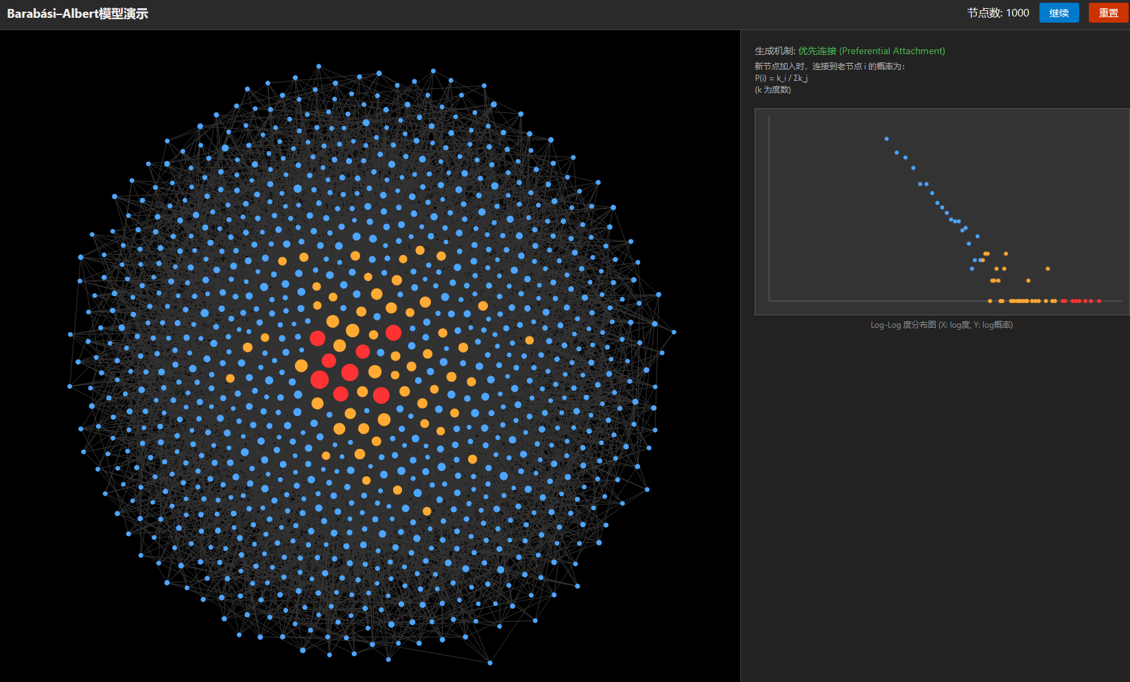
\[P(X=x) \approx p(x) \cdot \Delta x \approx p(x) \cdot \frac{dx}{dn} \cdot \Delta n = p(x) \cdot x \ln 2 \cdot 1 \propto x^{-1}\]

优先连接模型 (Barabási–Albert Model)

模型设定：

1. 增长：每个时间步 $t$ 加入一个新节点，带有 $m$ 条边。

2. 优先连接：新节点连接到已有节点 $i$ 的概率 $\Pi(k_i)$ 与节点 $i$ 的度数 $k_i$ 成正比：

   \[\Pi(k_i) = \frac{k_i}{\sum_j k_j}\]

理论分析

平均场近似推导：

设 $k_i(t)$ 是节点 $i$ 在时间 $t$ 的度数（视作连续变量）。 度数的变化率 $\frac{dk_i}{dt}$ 等于新节点连接到它的概率：

\[\frac{dk_i}{dt} = m \cdot \Pi(k_i) = m \cdot \frac{k_i}{\sum_j k_j}\]

由于每个时间步增加 $m$ 条边（即 $2m$ 个度），在时间 $t$ 时总度数 $\sum k_j \approx 2mt$。 代入方程：

\[\frac{dk_i}{dt} = m \frac{k_i}{2mt} = \frac{k_i}{2t}\]

分离变量积分： \(\frac{dk_i}{k_i} = \frac{dt}{2t} \implies \ln k_i = \frac{1}{2} \ln t + C\) 得到： \(k_i(t) = m \left( \frac{t}{t_i} \right)^{0.5}\) (其中 $t_i$ 是节点 $i$ 加入网络的时间，此时它的初始度数为 $m$)。

求度$K$分布 $P(k)$：

概率 $P(K = k(t) < k)$ 等价于 $P(t_{add} > \text{某时间})$。

由于节点是均匀时间间隔加入的，加入时间 $t_{add}$ 在 $[0, t]$ 上服从均匀分布，即 $P(t_{add} \leq \tau) = \tau/t$。

根据 $k = m (t/t_{add})^{0.5}$，解出 $t_{add} = t (m/k)^2$。

\[P(K < k) = P(t_{add} > t \frac{m^2}{k^2}) = 1 - P(t_{add} \leq t \frac{m^2}{k^2}) = 1 - \frac{t(m/k)^2}{t} = 1 - \frac{m^2}{k^2}\]

概率密度函数为累积分布函数的导数：

\[P(k) = \frac{d}{dk} \left( 1 - \frac{m^2}{k^2} \right) = 2m^2 k^{-3}\]

结论：度分布服从幂指数 $\alpha = 3$ 的幂律分布 $P(k) \propto k^{-3}$。

演示代码

力导向布局：

• 库仑力：点和点之间排斥
• 弹簧力：连边看作弹簧
• 摩擦力：速度衰减

<!DOCTYPE html>
<html lang="zh-CN">
  <head>
    <meta charset="UTF-8" />
    <title>幂律分布生成机制：优先连接 (BA模型) 可视化</title>
    <style>
      body {
        font-family: "Segoe UI", sans-serif;
        background: #1a1a1a;
        color: #eee;
        margin: 0;
        display: flex;
        flex-direction: column;
        height: 100vh;
        overflow: hidden;
      }
      header {
        padding: 10px 20px;
        background: #2a2a2a;
        border-bottom: 1px solid #444;
        display: flex;
        justify-content: space-between;
        align-items: center;
      }
      h1 {
        font-size: 18px;
        margin: 0;
      }
      .controls button {
        background: #007acc;
        border: none;
        color: white;
        padding: 5px 15px;
        cursor: pointer;
        border-radius: 3px;
        font-size: 14px;
        margin-left: 10px;
      }
      .controls button:hover {
        background: #005f9e;
      }
      .controls button.stop {
        background: #cc3300;
      }

      #main-container {
        display: flex;
        flex: 1;
        height: 100%;
      }

      /* 左侧网络视图 */
      #network-view {
        flex: 2;
        position: relative;
        border-right: 1px solid #444;
        background: #000;
      }
      canvas#netCanvas {
        display: block;
        width: 100%;
        height: 100%;
      }

      /* 右侧图表视图 */
      #chart-view {
        flex: 1;
        padding: 20px;
        display: flex;
        flex-direction: column;
        background: #222;
      }
      .stat-box {
        margin-bottom: 20px;
        font-size: 14px;
        color: #aaa;
      }
      .stat-value {
        color: #fff;
        font-weight: bold;
        font-size: 18px;
      }
      canvas#plotCanvas {
        background: #333;
        width: 100%;
        height: 300px;
        border: 1px solid #555;
      }
      .plot-label {
        text-align: center;
        font-size: 12px;
        margin-top: 5px;
        color: #888;
      }
    </style>
  </head>
  <body>
    <header>
      <h1>Barabási–Albert模型演示</h1>
      <div class="controls">
        <span id="node-count">节点数: 0</span>
        <button onclick="toggleSim()" id="btn-toggle">暂停</button>
        <button onclick="resetSim()" class="stop">重置</button>
      </div>
    </header>

    <div id="main-container">
      <div id="network-view">
        <canvas id="netCanvas"></canvas>
      </div>
      <div id="chart-view">
        <div class="stat-box">
          <div>生成机制: <span style="color: #4caf50">优先连接 (Preferential Attachment)</span></div>
          <div style="margin-top: 5px; font-size: 12px; line-height: 1.4">
            新节点加入时，连接到老节点 i 的概率为：<br />
            P(i) = k_i / Σk_j <br />
            (k 为度数)
          </div>
        </div>

        <canvas id="plotCanvas"></canvas>
        <div class="plot-label">Log-Log 度分布图 (X: log度, Y: log概率)</div>
      </div>
    </div>

    <script>
      /**
       * 简单的力导向图 + BA模型模拟
       */

      const canvas = document.getElementById("netCanvas");
      const ctx = canvas.getContext("2d");
      const pCanvas = document.getElementById("plotCanvas");
      const pCtx = pCanvas.getContext("2d");

      let width, height, pWidth, pHeight;

      // 模拟参数
      const MAX_POINTS = 1000;
      const M = 6; // 新节点每次产生 M 条边
      let nodes = [];
      let edges = [];
      let isRunning = true;
      let animationId;

      // 物理参数
      const REPULSION = 25;
      const SPRING_LENGTH = 100;
      const SPRING_K = 0.001;
      const CENTER_GRAVITY = 0.001; // 稍微拉向中心防止飞出
      const FRAC = 0.95; // 摩擦力

      class Node {
        constructor(id) {
          this.id = id;
          this.x = Math.random() * width;
          this.y = Math.random() * height;
          this.vx = 0;
          this.vy = 0;
          this.degree = 0;
          this.color = "#ccc";
          this.radius = 1;
        }

        get mass() {
          return Math.sqrt(this.degree);
        }

        update() {
          this.x += this.vx;
          this.y += this.vy;

          this.vx *= FRAC;
          this.vy *= FRAC;
        }

        draw() {
          // 根据度数调整大小和颜色 (可视化 Hub)
          const size = 1 + this.mass;
          this.radius = size;

          ctx.beginPath();
          ctx.arc(this.x, this.y, size, 0, Math.PI * 2);

          // 简单的热度图颜色
          if (this.mass > 9) ctx.fillStyle = "#ff3333"; // Super Hub
          else if (this.mass > 5) ctx.fillStyle = "#ffaa33"; // Hub
          else ctx.fillStyle = "#4da6ff"; // Normal

          ctx.fill();
        }
      }

      function resize() {
        width = canvas.width = canvas.offsetWidth;
        height = canvas.height = canvas.offsetHeight;
        pWidth = pCanvas.width = pCanvas.offsetWidth;
        pHeight = pCanvas.height = pCanvas.offsetHeight;
      }
      window.addEventListener("resize", resize);
      resize();

      function init() {
        nodes = [];
        edges = [];
        // 初始完全连接图
        const initialSize = 7;
        for (let i = 0; i < initialSize; i++) {
          nodes.push(new Node(i));
          // 放在中心附近
          nodes[i].x = width / 2 + (Math.random() - 0.5) * 50;
          nodes[i].y = height / 2 + (Math.random() - 0.5) * 50;
        }
        // 全连接
        for (let i = 0; i < initialSize; i++) {
          for (let j = i + 1; j < initialSize; j++) {
            addEdge(i, j);
          }
        }
        drawPlot();
      }

      function addEdge(sourceIdx, targetIdx) {
        edges.push({ source: sourceIdx, target: targetIdx });
        nodes[sourceIdx].degree++;
        nodes[targetIdx].degree++;
      }

      // 核心：优先连接算法
      function addNode() {
        if (nodes.length > MAX_POINTS) {
          // 限制节点总数防止卡顿
          document.getElementById("btn-toggle").innerText = "已达上限";
          return;
        }

        const newNodeIdx = nodes.length;
        const newNode = new Node(newNodeIdx);

        // 新节点从随机位置出生
        newNode.x = Math.random() * width;
        newNode.y = Math.random() * height;
        nodes.push(newNode);

        // 计算总度数
        let totalDegree = 0;
        for (let n of nodes) totalDegree += n.degree;

        // 选择 M 个已有节点进行连接
        // 使用轮盘赌算法 (Roulette Wheel Selection)
        let targets = [];
        let attempts = 0;

        while (targets.length < M && attempts < 100) {
          attempts++;
          const rand = Math.random() * totalDegree;
          let cumulative = 0;
          let selected = -1;

          for (let i = 0; i < nodes.length - 1; i++) {
            // 不包括自己
            cumulative += nodes[i].degree;
            if (cumulative >= rand) {
              selected = i;
              break;
            }
          }

          if (selected !== -1 && !targets.includes(selected)) {
            targets.push(selected);
          }
        }

        // 建立连接
        targets.forEach((targetIdx) => {
          addEdge(newNodeIdx, targetIdx);
        });

        document.getElementById("node-count").innerText = `节点数: ${nodes.length}`;
      }

      // 物理引擎步骤
      function physics() {
        // 1. 库仑力 (斥力)
        for (let i = 0; i < nodes.length; i++) {
          for (let j = i + 1; j < nodes.length; j++) {
            const dx = nodes[i].x - nodes[j].x;
            const dy = nodes[i].y - nodes[j].y;
            const distSq = dx * dx + dy * dy;
            if (distSq === 0) continue;
            const dist = Math.sqrt(distSq);
            const force = (REPULSION * nodes[i].mass * nodes[j].mass) / (distSq + 100);
            const fx = (dx / dist) * force;
            const fy = (dy / dist) * force;

            nodes[i].vx += fx / nodes[i].mass;
            nodes[i].vy += fy / nodes[i].mass;
            nodes[j].vx -= fx / nodes[j].mass;
            nodes[j].vy -= fy / nodes[j].mass;
          }

          // 重力向中心
          nodes[i].vx += (width / 2 - nodes[i].x) * CENTER_GRAVITY;
          nodes[i].vy += (height / 2 - nodes[i].y) * CENTER_GRAVITY;
        }

        // 2. 弹簧力
        for (let e of edges) {
          const u = nodes[e.source];
          const v = nodes[e.target];
          const dx = v.x - u.x;
          const dy = v.y - u.y;
          const dist = Math.sqrt(dx * dx + dy * dy);

          const force = (dist - SPRING_LENGTH) * SPRING_K;
          const fx = (dx / dist) * force;
          const fy = (dy / dist) * force;

          u.vx += fx / u.mass;
          u.vy += fy / u.mass;
          v.vx -= fx / v.mass;
          v.vy -= fy / v.mass;
        }

        // 3. 更新位置
        for (let n of nodes) n.update();
      }

      function drawNetwork() {
        ctx.clearRect(0, 0, width, height);

        // 画边
        ctx.strokeStyle = "#333";
        ctx.lineWidth = 1;
        ctx.beginPath();
        for (let e of edges) {
          const u = nodes[e.source];
          const v = nodes[e.target];
          ctx.moveTo(u.x, u.y);
          ctx.lineTo(v.x, v.y);
        }
        ctx.stroke();

        // 画点
        for (let n of nodes) n.draw();
      }

      // 绘制 Log-Log Plot
      function drawPlot() {
        // 统计度分布
        const frequencies = {};
        let maxDegree = 0;

        nodes.forEach((n) => {
          const d = n.degree;
          if (d === 0) return;
          if (!frequencies[d]) frequencies[d] = 0;
          frequencies[d]++;
          if (d > maxDegree) maxDegree = d;
        });

        pCtx.clearRect(0, 0, pWidth, pHeight);

        // 准备数据点: [log(k), log(P(k))]
        // 这里用 log(Frequency) 代替 log(P(k))，形状是一样的
        const points = [];
        for (let k in frequencies) {
          const x = Math.log10(parseInt(k));
          const y = Math.log10(frequencies[k]);
          const mass = Math.sqrt(parseInt(k));
          points.push({ x, y, mass });
        }

        if (points.length < 2) return;

        // 计算绘图范围
        const minX = 1;
        const maxX = Math.log10(maxDegree) * 1.05; // 留点余地

        // Y轴最大值通常是 log(节点总数) 或 log(count=1的度数)
        let maxY = 0;
        points.forEach((p) => {
          if (p.y > maxY) maxY = p.y;
        });
        maxY *= 1.1;

        const mapX = (val) => (val / maxX) * (pWidth - 40) + 20;
        const mapY = (val) => pHeight - 20 - (val / maxY) * (pHeight - 40);

        // 画坐标轴
        pCtx.strokeStyle = "#666";
        pCtx.beginPath();
        pCtx.moveTo(20, pHeight - 20);
        pCtx.lineTo(pWidth - 10, pHeight - 20); // X axis
        pCtx.moveTo(20, pHeight - 20);
        pCtx.lineTo(20, 10); // Y axis
        pCtx.stroke();

        // 画点

        points.forEach((p) => {
          if (p.mass > 9) pCtx.fillStyle = "#ff3333"; // Super Hub
          else if (p.mass > 5) pCtx.fillStyle = "#ffaa33"; // Hub
          else pCtx.fillStyle = "#4da6ff"; // Normal

          const px = mapX(p.x);
          const py = mapY(p.y);
          pCtx.beginPath();
          pCtx.arc(px, py, 3, 0, Math.PI * 2);
          pCtx.fill();
        });
      }

      // 主循环
      let frameCount = 0;
      function loop() {
        if (!isRunning) return;

        physics();
        drawNetwork();

        // 每隔几帧加一个节点
        if (frameCount % 5 === 0 && nodes.length < MAX_POINTS) {
          addNode();
          drawPlot();
        }

        systemEnergy = 0;
        nodes.forEach((n) => {
          systemEnergy += 0.5 * n.mass * (n.vx * n.vx + n.vy * n.vy);
        });

        if (MAX_POINTS == nodes.length && systemEnergy / MAX_POINTS < 1e-2) {
          toggleSim();
        }

        frameCount++;
        animationId = requestAnimationFrame(loop);
      }

      function toggleSim() {
        isRunning = !isRunning;
        const btn = document.getElementById("btn-toggle");
        btn.innerText = isRunning ? "暂停" : "继续";
        if (isRunning) loop();
      }

      function resetSim() {
        isRunning = false;
        cancelAnimationFrame(animationId);
        document.getElementById("btn-toggle").innerText = "暂停";
        init();
        isRunning = true;
        frameCount = 0;
        loop();
      }

      // 启动
      init();
      loop();
    </script>
  </body>
</html>

参数估计

错误做法：Log-Log 线性拟合

假设幂律分布为 $p(x) = C x^{-\alpha}$。

取对数：$\ln p(x) = -\alpha \ln x + \ln C$。

这看起来像线性方程 $y = ax + b$。然而，普通最小二乘法（OLS）有两个核心假设：

1. 误差服从正态分布。
2. 方差齐性（Homoscedasticity），即误差的方差是常数。

在幂律分布的尾部（大 $x$ 处），数据非常稀疏，往往只有 0 或 1 个样本。对这些计数取对数（特别是 $\ln 0$ 无意义，$\ln 1 = 0$）会导致极大的、非高斯的、且方差随 $x$ 剧烈变化的残差。这违背了 OLS 的假设，导致算出的 $\alpha$ 通常偏大（斜率更陡）。

标准流程

Clauset et al. 2009：

1. 使用 最大似然估计 计算 $\alpha$。
2. 使用 Kolmogorov-Smirnov (KS) 检验来确定数据是否真的符合幂律，以及确定 $x_{\min}$ 的截断位置。

最大似然估计（连续型）

设定： 设随机变量 $x$ 服从连续幂律分布，定义域为 $x \ge x_{\min}$，参数为 $\alpha > 1$。

求归一化常数 $C$

概率密度函数 (PDF) 必须满足全积分为 1：

\[\int_{x_{\min}}^{\infty} C x^{-\alpha} dx = 1\] \[C \left[ \frac{x^{-\alpha+1}}{-\alpha+1} \right]_{x_{\min}}^{\infty} = 1\]

由于 $\alpha > 1$，则 $x \to \infty$ 时项为 0：

\[C \left( 0 - \frac{x_{\min}^{1-\alpha}}{1-\alpha} \right) = 1 \implies C = \frac{\alpha - 1}{x_{\min}^{1-\alpha}}\]

将 $C$ 代回 PDF 表达式：

\[p(x) = \frac{\alpha-1}{x_{\min}^{1-\alpha}} x^{-\alpha} = \frac{\alpha-1}{x_{\min}} \left( \frac{x}{x_{\min}} \right)^{-\alpha}\]

构建对数似然函数

假设观测 $n$ 个独立的数据点 $x_1, x_2, …, x_n$（其中所有 $x_i \ge x_{\min}$）。 似然函数 $L(\alpha)$ 为所有样本概率密度的乘积：

\[L(\alpha) = \prod_{i=1}^{n} p(x_i) = \prod_{i=1}^{n} \frac{\alpha-1}{x_{\min}} \left( \frac{x_i}{x_{\min}} \right)^{-\alpha}\]

为了方便求导，取自然对数 $\mathcal{L}(\alpha) = \ln L(\alpha)$：

\[\mathcal{L}(\alpha) = \sum_{i=1}^{n} \left[ \ln(\alpha-1) - \ln x_{\min} - \alpha (\ln x_i - \ln x_{\min}) \right]\] \[\mathcal{L}(\alpha) = n \ln(\alpha-1) - n \ln x_{\min} - \alpha \sum_{i=1}^{n} \ln \left( \frac{x_i}{x_{\min}} \right)\]

求极大值

对 $\alpha$ 求偏导，并令其为 0：

\[\frac{\partial \mathcal{L}}{\partial \alpha} = \frac{n}{\alpha-1} - \sum_{i=1}^{n} \ln \left( \frac{x_i}{x_{\min}} \right) = 0\] \[\hat{\alpha} = 1 + n \left[ \sum_{i=1}^{n} \ln \frac{x_i}{x_{\min}} \right]^{-1}\]

标准误 (Standard Error)

为了衡量估计的波动性，我们需要看对数似然函数的二阶导数。二阶导数描述了函数在极值附近的弯曲程度（曲率）。

\[\frac{\partial^2 \mathcal{L}}{\partial \alpha^2} = \frac{\partial}{\partial \alpha} \left( \frac{n}{\alpha - 1} - \sum_{i=1}^{n} \ln \left( \frac{x_i}{x_{\min}} \right) \right) = -\frac{n}{(\alpha - 1)^2}\]

Fisher 信息量 $I_n(\alpha)$ 定义为对数似然函数二阶导数的期望值的负数：

\[I_n(\alpha) = - E \left[ \frac{\partial^2 \mathcal{L}}{\partial \alpha^2} \right]\]

将刚才算出的二阶导数代入：

\[I_n(\alpha) = - E \left[ -\frac{n}{(\alpha - 1)^2} \right] = E \left[ \frac{n}{(\alpha - 1)^2} \right]\]

由于 $\frac{n}{(\alpha - 1)^2}$ 是一个常数（相对于随机变量 $x$ 而言，它不包含 $x$），所以它的期望就是它本身：

\[I_n(\alpha) = \frac{n}{(\alpha - 1)^2}\]

物理意义：Fisher 信息量越大，说明似然函数的峰越尖，估计越准，方差越小。

对于大样本（$n \to \infty$），极大似然估计量 $\hat{\alpha}$ 渐进无偏。

对于无偏估计量，方差 $\text{Var}(\hat{\alpha})$ 的Cramer-Rao下界 由 Fisher 信息量的倒数给出：

\[\text{Var}(\hat{\alpha}) \approx \frac{1}{I_n(\alpha)}\]

将 $I_n(\alpha)$ 代入：

\[\text{Var}(\hat{\alpha}) \approx \frac{1}{\frac{n}{(\alpha - 1)^2}} = \frac{(\alpha - 1)^2}{n}\] \[\sigma = \frac{\hat{\alpha} - 1}{\sqrt{n}}\]

最大似然估计（连续型修正）

虽然观测到的度分布 $x$ 是离散的整数（$x \in {x_{\min}, x_{\min}+1, \dots}$），但我们可以假设这些离散整数是由底层的连续实数 $y$ 经过四舍五入得到的。

1. 区间映射： 一个离散整数 $x$ 代表了连续区间 $[x - \frac{1}{2}, x + \frac{1}{2})$ 内的所有实数。

2. 截断位置的修正： 如果我们设定的离散截断点是 $x_{\min}$（即我们要分析所有 $\ge x_{\min}$ 的整数），那么在连续空间中，这意味着我们涵盖了从 $x_{\min}$ 所代表的区间下界开始的所有数据。 因此，连续模型的真实下界 $y_{\min}$ 应该是： \(y_{\min} = x_{\min} - \frac{1}{2}\)

将上述代换代入连续 MLE 公式：

\[\hat{\alpha} \simeq 1 + n \left[ \sum_{i=1}^{n} \ln \left( \frac{x_i}{x_{\min} - \frac{1}{2}} \right) \right]^{-1}\]

最大似然估计（离散型）

Barabási–Albert (BA) 模型生成的网络度分布是离散整数（$k=1, 2, 3, …$）。对于离散数据，使用连续近似会引入偏差，特别是当 $x_{\min}$ 较小的时候（例如 $x_{\min} < 6$）。连续估计量得到的 $\alpha$ 通常会比真实值偏低。

概率质量函数 (PMF)

离散幂律分布遵循 Zipf 分布（或称为 Zeta 分布）。 设随机变量 $x$ 取整数值 $x \in {x_{\min}, x_{\min}+1, \dots}$。

\[p(x) = \frac{x^{-\alpha}}{Z}\]

其中 $Z$ 是归一化常数。

归一化常数 (Hurwitz Zeta 函数)

概率之和必须为 1：

\[\sum_{k=x_{\min}}^{\infty} \frac{k^{-\alpha}}{Z} = 1 \implies Z = \sum_{k=x_{\min}}^{\infty} k^{-\alpha}\]

右边的级数正是 Hurwitz Zeta 函数，记作 $\zeta(\alpha, x_{\min})$：

\[\zeta(\alpha, x_{\min}) = \sum_{n=0}^{\infty} (n + x_{\min})^{-\alpha}\]

因此，离散幂律分布的 PMF 为：

\[p(x) = \frac{x^{-\alpha}}{\zeta(\alpha, x_{\min})}\]

对数似然函数 (Log-Likelihood)

假设有 $n$ 个观测数据 $x_1, x_2, \dots, x_n$。

似然函数 $L(\alpha)$ 为：

\[L(\alpha) = \prod_{i=1}^{n} \frac{x_i^{-\alpha}}{\zeta(\alpha, x_{\min})} = \frac{\prod x_i^{-\alpha}}{[\zeta(\alpha, x_{\min})]^n}\]

取对数似然 $\mathcal{L}(\alpha) = \ln L(\alpha)$：

\[\mathcal{L}(\alpha) = -\alpha \sum_{i=1}^{n} \ln x_i - n \ln \zeta(\alpha, x_{\min})\]

极大化

对 $\alpha$ 求导并令其为 0：

\[\frac{\partial \mathcal{L}}{\partial \alpha} = -\sum_{i=1}^{n} \ln x_i - n \frac{\partial}{\partial \alpha} \ln \zeta(\alpha, x_{\min}) = 0\]

这里涉及到 Zeta 函数的导数。令 $\zeta’(\alpha, x_{\min})$ 为 $\zeta$ 对 $\alpha$ 的导数，则 $\frac{\partial}{\partial \alpha} \ln \zeta = \frac{\zeta’}{\zeta}$。 方程变为：

\[-\sum_{i=1}^{n} \ln x_i - n \frac{\zeta'(\alpha, x_{\min})}{\zeta(\alpha, x_{\min})} = 0\]

整理得到 MLE 的条件方程：

\[\frac{\zeta'(\alpha, x_{\min})}{\zeta(\alpha, x_{\min})} = -\frac{1}{n} \sum_{i=1}^{n} \ln x_i\]

离散情况下的 $\alpha$ 没有解析解。

可以使用数值优化算法（如牛顿法或 Brent 方法）来最大化对数似然函数 $\mathcal{L}(\alpha)$，从而找到最优的 $\hat{\alpha}$。

关于 $x_{\min}$ 的选择：KS检验

为什么 $x_{\min}$ 不是数据的最小值?

因为绝大多数现实数据（甚至包括模拟数据），并不是从第一个数字开始就完美遵循幂律的。

数学上的幂律分布 $P(x) \propto x^{-\alpha}$ 往往描述的是系统在规模较大时的行为。

如果强行把 $x_{\min}$ 设为观测最小值，会导致严重的模型偏差。

即使是优先连接（BA）模型，虽然理论上说生成了无标度网络，但其解析解通常是在 $k \to \infty$（度很大）时才完美趋近于 $k^{-3}$。在度数较小（例如 $k=6, 7, 8$）时，由于有限尺寸或初始条件的影响，分布往往会发生偏离。

$x_{\min}$ 不是数据的最小值，而是幂律模型的有效起始值。

解决方法：自动试探，把前面的非幂律部分切掉，只保留后面的部分进行拟合。

我们不能预先知道幂律从哪里开始（即 $x_{\min}$ 是多少）。Clauset 方法的核心逻辑是：

1. 将数据中的每一个唯一值尝试作为 $x_{\min}$。
2. 对于每一个假设的 $x_{\min}$，利用上述 MLE 公式计算对应的 $\alpha$。

3. 计算理论累积分布函数 (CDF) 与 实际数据经验 CDF 之间的距离（Kolmogorov-Smirnov 统计量 $D$）：

   \[D = \max_{x \ge x_{\min}} | S(x) - P(x) |\]

   其中 $S(x)$ 是数据的累积频率，$P(x)$ 是拟合出的幂律模型的 CDF。

4. 选择使 $D$ 最小的那个 $x_{\min}$。

代码

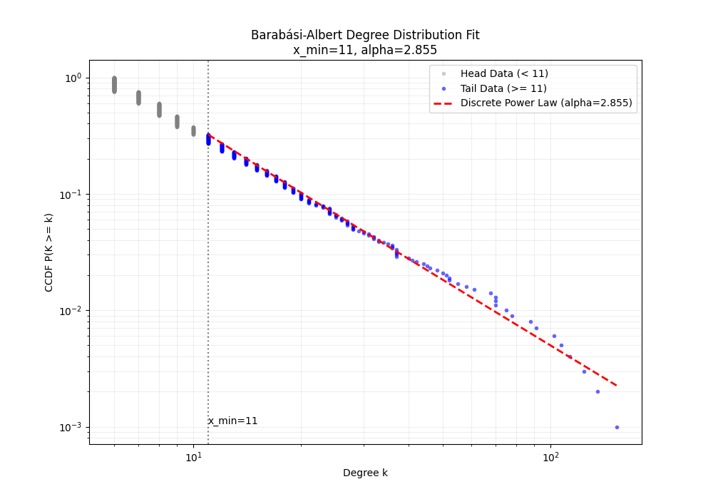
使用连续型修正的公式计算 $\alpha$ 的估计值，使用 Zeta 分布 进行 KS检验。

可视化CCDF的表现：

CCDF 是累积求和：$P(K \ge k) = \sum_{x=k}^{\infty} P(x)$。

积分（求和）具有平滑的效果。它把尾部那些极其稀疏的数据累加起来，消除了剧烈的波动（斜率为 $1-\alpha$）。

Using the CCDF is a far superior method for visualizing power-law data.

import numpy as np
import matplotlib.pyplot as plt
from scipy.special import zeta

degrees = [135,153,88,102,124,70,78,107,113,68,75,70,55,70,58,23,52,33,46,34,40,36,51,42,30,28,33,91,48,37,28,44,61,21,37,35,31,50,32,17,36,32,21,24,18,41,29,14,37,27,27,27,21,18,24,52,24,28,37,27,45,27,25,12,18,24,16,12,32,19,25,26,18,37,26,28,18,19,19,23,16,13,24,15,25,24,19,13,20,18,21,22,13,31,11,9,14,12,26,26,30,10,18,13,16,16,19,20,13,17,18,11,15,36,24,17,18,20,24,11,28,16,21,20,16,19,10,19,20,14,22,24,19,12,20,18,18,23,19,20,14,25,15,16,18,18,22,14,19,14,23,16,20,15,9,11,14,20,11,16,20,12,12,12,11,15,15,13,16,17,14,9,20,11,17,19,12,14,21,14,6,13,14,15,14,9,11,16,11,21,12,13,15,17,17,11,8,11,14,17,8,10,11,9,15,17,6,15,20,17,16,12,13,12,6,11,16,10,11,11,15,9,9,16,9,10,9,12,8,11,9,12,14,9,10,9,14,8,10,10,11,8,14,13,14,13,15,10,17,7,10,14,12,10,8,18,8,13,12,8,13,7,11,13,11,13,8,9,17,9,11,12,18,10,8,15,12,7,15,6,14,11,12,8,15,10,15,10,12,9,10,12,13,11,8,12,9,9,7,11,13,12,13,11,7,12,9,8,10,12,12,6,14,15,11,9,9,12,9,15,15,8,7,10,15,10,9,17,9,13,9,11,10,8,9,12,6,9,8,14,11,11,11,8,12,9,10,14,13,11,11,13,11,12,12,11,8,9,7,8,9,12,8,9,13,7,8,11,12,17,9,7,11,9,10,10,11,12,11,8,10,7,11,9,8,9,11,8,10,16,8,8,12,11,9,8,9,14,8,8,6,8,9,9,6,9,7,9,8,9,10,8,9,7,7,8,9,7,10,8,9,10,7,7,17,7,9,8,10,13,12,10,7,13,9,8,7,14,11,10,8,13,10,9,10,9,13,8,8,11,7,8,9,7,8,11,13,6,9,10,8,9,9,9,8,10,9,6,9,8,6,11,7,10,10,7,8,6,8,7,9,8,8,10,9,13,7,9,8,8,8,9,8,7,8,7,7,8,7,12,8,9,11,7,6,9,11,7,7,6,10,6,7,8,10,9,10,8,7,11,8,8,6,7,7,10,11,10,12,10,8,6,6,7,9,7,10,8,8,9,6,8,10,7,6,6,6,10,6,8,16,7,7,7,9,7,9,7,8,9,8,8,6,6,11,7,6,8,7,9,9,12,7,9,11,8,8,7,7,6,8,6,7,7,8,10,8,9,7,12,7,6,11,9,8,8,6,7,8,11,7,8,8,6,7,7,9,7,6,10,6,7,6,8,9,9,6,7,7,8,10,6,6,6,8,6,8,8,7,9,6,8,6,6,6,7,6,8,7,6,6,6,8,6,7,9,8,6,6,11,6,6,9,6,8,8,7,8,9,7,6,6,6,8,7,10,7,8,8,8,7,8,6,7,9,7,8,6,10,7,8,9,7,6,6,7,9,7,8,8,8,7,8,6,9,6,6,9,7,7,8,10,7,7,6,6,7,7,9,9,6,7,7,6,6,6,7,7,8,6,6,6,8,6,8,10,6,7,7,7,6,7,6,7,7,6,6,7,8,9,6,7,8,7,6,8,9,7,7,8,6,8,7,8,6,6,7,6,6,9,7,9,6,7,7,7,6,6,6,9,6,6,7,7,6,8,6,7,8,7,6,6,8,6,7,7,7,6,6,6,7,8,8,6,7,7,6,8,7,7,6,8,6,8,6,7,7,6,8,6,6,7,8,6,8,9,6,8,7,6,6,6,7,6,6,6,6,6,6,6,8,6,6,8,6,7,6,6,7,7,6,6,6,6,7,6,6,6,7,7,6,6,6,6,6,6,7,6,8,6,6,7,7,6,6,6,6,7,8,6,6,6,6,6,8,6,6,7,6,7,6,6,8,6,8,6,6,6,7,6,7,6,7,7,6,7,6,7,7,6,6,6,6,6,6,7,6,6,7,6,6,7,6,7,7,6,7,6,6,7,7,6,7,6,6,6,6,6,6,6,7,6,6,6,6,6,7,6,6,6,6,6,8,7,6,6,6,6,6,7,6,6,6,6,6,6,7,6,6,6,6,6,6,6,6,6,6,6,6,6,7,6,6,6,6,6,6,6,6,6,6,6,6,6,6,6,6,6,6,6,6,6,6,6,6,6,6,6,6,6]

data = np.array(degrees)
data.sort()

def calculate_alpha(data_subset, x_min):
    n = len(data_subset)
    if n <= 1: 
        return None
    
    sum_ln = np.sum(np.log(data_subset / (x_min - 0.5)))
    if sum_ln <= 0: 
        return None
    
    alpha = 1 + n * (1.0 / sum_ln)
    return alpha

def calculate_standard_error(alpha, n):
    if n <= 0: 
        return 0
    return (alpha - 1) / np.sqrt(n)

def ks_test(data_subset, x_min, alpha):
    unique_data, counts = np.unique(data_subset, return_counts=True)
    empirical_cdf = np.cumsum(counts) / len(data_subset)
    
    # 理论 CDF: P(X <= x) = 1 - zeta(alpha, x+1)/zeta(alpha, xmin)
    Z = zeta(alpha, x_min)
    theoretical_cdf = []
    for x in unique_data:
        p_le_x = 1 - (zeta(alpha, x + 1) / Z)
        theoretical_cdf.append(p_le_x)
    
    D = np.max(np.abs(empirical_cdf - np.array(theoretical_cdf)))
    return D

def find_x_min(data):
    unique_values = np.unique(data)
    # 排除太大的 x_min 保证尾部有足够样本
    candidate_x_mins = unique_values[unique_values < np.max(unique_values)/3] 

    best_xmin = None
    best_alpha = None
    best_sigma = None
    min_D = float('inf')
    results = []

    print(f"{'x_min':<8} {'Approx Alpha':<15} {'Sigma (Err)':<15} {'KS (D)':<10} {'N_tail'}")
    print("-" * 65)

    for x_min in candidate_x_mins:
        subset = data[data >= x_min]
        n = len(subset)
        # 样本量不能太小
        if n < 30: 
            continue

        alpha = calculate_alpha(subset, x_min)
        if alpha is None: continue
        sigma = calculate_standard_error(alpha, n)
        D = ks_test(subset, x_min, alpha)
        results.append((x_min, alpha, sigma, D, n))
        print(f"{x_min:<8} {alpha:<15.4f} {sigma:<15.4f} {D:<10.4f} {n}")

        # 更新最优解
        if D < min_D:
            min_D = D
            best_xmin, best_alpha, best_sigma = x_min, alpha, sigma

    print("-" * 65)
    print("最优结果:")
    print(f"x_min = {best_xmin}, alpha = {best_alpha:.8f}, sigma = {best_sigma:.4f}, KS_Distance = {min_D:.4f}")
    return best_xmin, best_alpha

def plot_result(data, x_min, alpha):
    # 1. 准备全局数据
    data_sorted = np.sort(data)
    n_total = len(data_sorted)
    # 计算全局经验 CCDF: P(X >= x)
    # y 轴坐标为: 1.0, ..., 2/N, 1/N
    y_all = 1.0 - np.arange(n_total) / n_total
    
    # 2. 将数据切分为两部分：头部 (< x_min) 和 尾部 (>= x_min)
    mask_tail = data_sorted >= x_min
    mask_head = ~mask_tail  # 取反，即 < x_min 的部分
    
    x_head = data_sorted[mask_head]
    y_head = y_all[mask_head]
    
    x_tail = data_sorted[mask_tail]
    y_tail = y_all[mask_tail]
    
    # 3. 计算理论拟合线
    # 要画在全局图上，必须乘以尾部数据的比例 (n_tail / n_total)
    tail_ratio = len(x_tail) / n_total
    
    # 生成理论线的 x 坐标 (对数刻度)
    x_theory = np.unique(np.logspace(np.log10(x_min), np.log10(max(data)), 100).astype(int))
    
    # 计算 Zeta 归一化常数
    Z = zeta(alpha, x_min)
    
    # 计算理论 y 值并缩放
    y_theory = []
    for xi in x_theory:
        # P(X >= xi | X >= xmin)
        p_conditional = zeta(alpha, xi) / Z
        # 缩放到全局比例
        y_theory.append(p_conditional * tail_ratio)
    
    # 4. 绘图
    plt.figure(figsize=(10, 7))
    
    # 头部数据 (灰色或浅色表示，显示被丢弃的部分)
    plt.loglog(x_head, y_head, 'o', color='gray', alpha=0.4, markersize=4, 
               markeredgewidth=0, label=f'Head Data (< {x_min})')
    
    # 尾部数据 (蓝色表示)
    plt.loglog(x_tail, y_tail, 'bo', alpha=0.6, markersize=4, 
               markeredgewidth=0, label=f'Tail Data (>= {x_min})')
    
    # 理论拟合线 (红色虚线)
    plt.loglog(x_theory, y_theory, 'r--', linewidth=2, 
               label=f'Discrete Power Law (alpha={alpha:.3f})')
    
    # 竖线指示 x_min
    plt.axvline(x=x_min, color='black', linestyle=':', alpha=0.5)
    plt.text(x_min, min(y_all), f'x_min={x_min}', verticalalignment='bottom')

    # label & title
    plt.xlabel('Degree k')
    plt.ylabel('CCDF P(K >= k)')
    plt.title(f'Barabási-Albert Degree Distribution Fit\nx_min={x_min}, alpha={alpha:.3f}')
    plt.legend()
    plt.grid(True, which="both", linestyle='-', alpha=0.2)
    
    plt.savefig("BA_MLE.png")

best_xmin, best_alpha = find_x_min(data)
plot_result(data, best_xmin, best_alpha)

运行结果

x_min    Approx Alpha    Sigma (Err)     KS (D)     N_tail
-----------------------------------------------------------------
6        2.7645          0.0558          0.0177     1000
7        2.7951          0.0654          0.0198     753
8        2.8548          0.0758          0.0189     598
9        2.8278          0.0846          0.0135     467
10       2.7983          0.0929          0.0230     375
11       2.8550          0.1034          0.0131     322
12       2.8343          0.1118          0.0159     269
13       2.8282          0.1205          0.0182     230
14       2.8504          0.1302          0.0214     202
15       2.8625          0.1396          0.0250     178
16       2.8730          0.1490          0.0293     158
17       2.8941          0.1589          0.0363     142
18       2.8941          0.1681          0.0404     127
19       2.8542          0.1752          0.0321     112
20       2.8433          0.1834          0.0335     101
21       2.7786          0.1885          0.0583     89
22       2.7840          0.1970          0.0613     82
23       2.8674          0.2101          0.0395     79
24       2.9253          0.2223          0.0499     75
25       2.8326          0.2256          0.0450     66
26       2.8533          0.2354          0.0494     62
27       2.8623          0.2445          0.0535     58
28       2.8220          0.2503          0.0556     53
29       2.7593          0.2539          0.0704     48
30       2.8327          0.2673          0.0630     47
31       2.8663          0.2782          0.0679     45
32       2.8949          0.2890          0.0728     43
33       2.8696          0.2956          0.0769     40
34       2.8800          0.3050          0.0815     38
35       2.9362          0.3183          0.0942     37
36       2.9927          0.3321          0.1188     36
37       2.9290          0.3358          0.1007     33
-----------------------------------------------------------------
最优结果:
x_min = 11, alpha = 2.85501815, sigma = 0.1034, KS_Distance = 0.0131

和powerlaw包交叉验证

import powerlaw
fit = powerlaw.Fit(degrees, discrete=True)
print("MLE alpha =", fit.alpha)

Calculating best minimal value for power law fit
MLE alpha = 2.8550181506760337

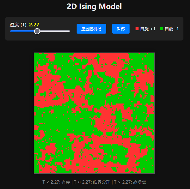
Ising 模型 (Ising Model)

这是一个描述铁磁性的统计力学模型。

生成机制：相互作用 vs 热扰动

• 相互作用 (Order)：系统由网格（Lattice）组成，每个节点有一个自旋 $\sigma_i \in {+1, -1}$。相邻的自旋倾向于方向一致（同向排列能量更低）。
• 热扰动 (Disorder)：环境温度 $T$ 提供热能，倾向于让自旋随机翻转。
• 相变：当有序倾向（耦合强度 $J$）与无序倾向（温度 $k_B T$）势均力敌时，系统会发生相变。

数学性质

• 哈密顿量 (能量函数)：

  \[H(\sigma) = -J \sum_{\langle i, j \rangle} \sigma_i \sigma_j\]

  其中 $\langle i, j \rangle$ 表示相邻节点，$J>0$ 表示铁磁性。

• Boltzmann 分布：系统处于某一状态的概率由 $P(\sigma) \propto e^{-H(\sigma)/k_B T}$ 决定。

• 临界点 (Critical Point)： 在临界温度 $T_c$（对于 2D 正方晶格，$T_c \approx 2.269 J/k_B$），相关长度（Correlation Length）$\xi$ 趋于无穷大：

  \[\xi \propto |T - T_c|^{-\nu}\]

• 幂律涌现：在 $T = T_c$ 时，自旋簇（即连在一起的同向区域）的大小 $s$ 服从幂律分布：

  \[P(s) \propto s^{-\tau}\]

  这体现了标度不变性 (Scale Invariance)：系统中存在各种大小的“岛屿”，从小如像素到大如整个系统，没有特征尺度。

相关长度

在统计物理中，相关长度 (Correlation Length, $\xi$) 是一个衡量系统中某一点的状态能够在多大范围内影响或关联到其他点状态的物理量。

自旋之间的关联性通常用关联函数 (Correlation Function) $G(r)$ 来描述，表示两个相距 $r$ 的自旋 $\sigma_0$ 和 $\sigma_r$ 方向一致的程度（减去平均磁化强度的背景后）。

在非临界温度下，关联函数通常呈指数衰减：

\[G(r) \sim e^{-r / \xi}\]

这里的 $\xi$ 就是相关长度。

• 当距离 $r < \xi$ 时，两个自旋的状态高度相关。
• 当距离 $r > \xi$ 时，关联迅速消失，变得不再相关。

1. 高温 ($T \gg T_c$)：热扰动剧烈，自旋随机翻转。$\xi$ 非常小（接近 0）。只有紧挨着的邻居有一点点关系，稍远一点就完全随机了。
2. 低温 ($T \ll T_c$)：系统处于有序态（比如全红或全绿）。虽然整体有序，但在热力学涨落的意义上，$\xi$ 也是有限的。
3. 临界温度 ($T \approx T_c$)：这是最神奇的时刻。$\xi$ 趋向于无穷大 ($\xi \to \infty$)。
   • 指数衰减变成了幂律衰减 ($G(r) \sim r^{-\eta}$)。
   • 这意味着，系统中某个点的微小扰动理论上可以影响到无限远处的其他点。整个系统在所有尺度上都变得连通了。这也是为什么在临界点能看到无论放大多少倍都相似的分形结构。

模拟

Metropolis 算法

核心目的：模拟自然界如何在热平衡状态下选择它的状态。

寻找能量最低点，但偶尔也会有热力学涨落。

自然的法则：

1. 能量越低越好：系统倾向于处于低能态

2. 自然界是随机的：由于温度 $T$ 的存在，系统并不总是待在能量最低状态，而是以一定的概率分布在各种状态中。这个概率由 Boltzmann 分布 决定：

   \[P(\text{state}) \propto e^{-E(\text{state}) / k_B T}\]

困难：要算出这个概率 $P$，分母是所有可能状态的总和（配分函数 $Z$）。对于一个 $100 \times 100$ 的网格，状态总数 $2^{10000}$ 是天文数字。

Metropolis： 不需要知道绝对概率，只需要知道相对概率。如果状态 A 变成状态 B，能量变了 $\Delta E$，可以只根据 $\Delta E$ 来决定是否允许这次变化。

Metropolis 算法是一个迭代过程（Monte Carlo 方法），步骤如下：

1. 当前状态：假设系统处于状态 $\mu$, 随机选一个自旋（比如朝上 $+1$）。
2. 尝试改变：尝试把它翻转（从 $+1$ 变 $-1$），得到新状态 $\nu$。
3. 计算能量差：计算翻转前后的能量变化： \(\Delta E = E_{\text{new}} - E_{\text{old}}\)
4. 审判：
   • 情况 A：能量降低 ($\Delta E \leq 0$)
     • 这意味着系统变得更稳定了。
     • 决定：100% 接受这次翻转。
   • 情况 B：能量升高 ($\Delta E > 0$)
     • 这意味着系统变得更混乱、不稳定了。
     • 决定：以一定的概率接受。这个概率是： \(P_{\text{accept}} = e^{-\frac{\Delta E}{k_B T}}\)

// 1. 尝试改变：假设 grid[idx] 翻转
// 2. 计算能量差
// 在 Ising 模型中，翻转一个自旋带来的能量变化只和它的邻居有关
// dE = 2 * J * s * (neighbors_sum)
const dE = 2 * J * s * (left + right + up + down);

// 3. 判据
if (dE <= 0) {
    // 情况 A: 能量降低，无条件接受
    grid[idx] = -s; 
} else {
    // 情况 B: 能量升高，按概率接受 (Boltzmann 因子)
    if (Math.random() < Math.exp(-dE / T)) {
        grid[idx] = -s;
    }
}

Metropolis 算法通过细致平衡 (Detailed Balance) 原理，保证了当模拟运行足够长时间后，系统出现某一状态的概率，严格等于统计力学计算出的理论概率。

代码

此代码可视化二维 Ising 模型在不同温度下的状态。

<!DOCTYPE html>
<html lang="zh">
<head>
    <meta charset="UTF-8">
    <title>Ising Model</title>
    <style>
        body {
            font-family: sans-serif;
            background-color: #111;
            color: #eee;
            display: flex;
            flex-direction: column;
            align-items: center;
            margin: 0;
            padding: 20px;
        }
        
        .container {
            position: relative;
            margin-top: 20px;
        }

        /* 关键：CSS控制显示大小，image-rendering保证放大不模糊 */
        canvas {
            width: 400px;         /* 显示宽度 */
            height: 400px;        /* 显示高度 */
            image-rendering: pixelated; /* 像素化放大，关键 */
            image-rendering: crisp-edges;
            border: 2px solid #555;
            box-shadow: 0 0 20px rgba(0,0,0,0.5);
            background-color: #000; /* 默认黑色背景 */
        }

        .controls {
            background: #222;
            padding: 15px;
            border-radius: 8px;
            margin-bottom: 20px;
            display: flex;
            gap: 20px;
            align-items: center;
            flex-wrap: wrap;
            justify-content: center;
        }

        input[type=range] { width: 200px; cursor: pointer; }
        
        button {
            padding: 8px 16px;
            background-color: #007bff;
            color: white;
            border: none;
            border-radius: 4px;
            cursor: pointer;
        }
        button:hover { background-color: #0056b3; }
        
        .legend { font-size: 0.9em; display: flex; gap: 15px; }
        .dot { width: 10px; height: 10px; display: inline-block; margin-right: 5px; }
    </style>
</head>
<body>

    <h2>2D Ising Model</h2>

    <div class="controls">
        <div>
            <label>温度 (T): <span id="tempDisplay" style="color:yellow; font-weight:bold;">2.27</span></label>
            <br>
            <input type="range" id="tempSlider" min="0.1" max="5.0" step="0.01" value="2.27">
        </div>
        <button onclick="resetGrid()">重置随机场</button>
        <button onclick="togglePause()" id="pauseBtn">暂停</button>
        
        <div class="legend">
            <div><span class="dot" style="background:#FF3333"></span>自旋 +1</div>
            <div><span class="dot" style="background:#00CC00"></span>自旋 -1</div>
        </div>
    </div>

    <div class="container">
        <!-- 关键：物理分辨率设为 100x100，与网格大小一致 -->
        <canvas id="simCanvas" width="100" height="100"></canvas>
    </div>
    
    <p style="color:#888; font-size:0.9em; text-align:center;">
        T < 2.27: 有序 | T ≈ 2.27: 临界分形 | T > 2.27: 热噪点
    </p>

<script>
    // --- 参数配置 ---
    const GRID_SIZE = 100; // 网格尺寸
    let T = 2.27;          // 温度
    const J = 1.0;         // 交换相互作用强度

    // --- 状态变量 ---
    const canvas = document.getElementById('simCanvas');
    const ctx = canvas.getContext('2d');
    
    // 使用一维数组存储二维网格，性能更好
    // grid[y * GRID_SIZE + x]
    let grid = new Int8Array(GRID_SIZE * GRID_SIZE); 
    
    // 创建图像缓冲区 (Image Buffer)
    // 这是一个 100x100 的图像数据，每个点对应一个像素
    const imgData = ctx.createImageData(GRID_SIZE, GRID_SIZE);
    // 使用 32位视图操作像素，比操作 8位数组快 4倍
    // 每个像素是 0xAABBGGRR (Alpha, Blue, Green, Red)
    const buf32 = new Uint32Array(imgData.data.buffer);

    let isRunning = true;
    let frameId;

    // --- 颜色定义 (ABGR 格式, 因为是小端序) ---
    // Red: Alpha=FF(255), B=00, G=33, R=FF -> 0xFF0033FF
    const COLOR_UP = 0xFF3333FF;   // 红色 (自旋 +1)
    // Green: Alpha=FF(255), B=00, G=CC, R=00 -> 0xFF00CC00
    const COLOR_DOWN = 0xFF00CC00; // 绿色 (自旋 -1)

    // --- 初始化 ---
    function init() {
        // 绑定滑块
        const slider = document.getElementById('tempSlider');
        const display = document.getElementById('tempDisplay');
        slider.oninput = function() {
            T = parseFloat(this.value);
            display.innerText = T.toFixed(2);
        };

        resetGrid();
        loop();
    }

    function resetGrid() {
        for (let i = 0; i < grid.length; i++) {
            grid[i] = Math.random() > 0.5 ? 1 : -1;
        }
    }

    function togglePause() {
        isRunning = !isRunning;
        document.getElementById('pauseBtn').innerText = isRunning ? "暂停" : "继续";
        if (isRunning) loop();
    }

    // --- 核心物理引擎 (Metropolis 算法) ---
    function updatePhysics() {
        // 每帧尝试翻转 N次，保证演化速度
        const steps = GRID_SIZE * GRID_SIZE; 

        for (let k = 0; k < steps; k++) {
            // 随机选点
            const x = (Math.random() * GRID_SIZE) | 0; // | 0 是快速取整
            const y = (Math.random() * GRID_SIZE) | 0;
            const idx = y * GRID_SIZE + x;
            
            const s = grid[idx];

            // 周期性边界条件 (取模运算的快速写法)
            const left  = grid[y * GRID_SIZE + (x - 1 + GRID_SIZE) % GRID_SIZE];
            const right = grid[y * GRID_SIZE + (x + 1) % GRID_SIZE];
            const up    = grid[((y - 1 + GRID_SIZE) % GRID_SIZE) * GRID_SIZE + x];
            const down  = grid[((y + 1) % GRID_SIZE) * GRID_SIZE + x];

            // 计算能量差 dE = 2 * J * s * (Neighbors)
            const dE = 2 * J * s * (left + right + up + down);

            // Metropolis 判据
            if (dE <= 0 || Math.random() < Math.exp(-dE / T)) {
                grid[idx] = -s; // 翻转
            }
        }
    }

    // --- 渲染引擎 ---
    function draw() {
        // 直接更新 32位 buffer，速度极快
        for (let i = 0; i < grid.length; i++) {
            // 如果是 1 用红色，否则用绿色
            buf32[i] = (grid[i] === 1) ? COLOR_UP : COLOR_DOWN;
        }
        // 将数据一次性推送到 Canvas
        ctx.putImageData(imgData, 0, 0);
    }

    // --- 动画循环 ---
    function loop() {
        if (!isRunning) return;

        updatePhysics();
        draw();
        
        frameId = requestAnimationFrame(loop);
    }

    // 启动
    init();

</script>
</body>
</html>

细致平衡原理

细致平衡(Detailed Balance)是马尔可夫链 (Markov Chain) 收敛到平稳分布的一个充分条件。

想象有两个房间 A 和 B，里面都有人。

• 全局平衡 (Global Balance)：指的是房间 A 的总人数不变，房间 B 的总人数也不变。但这并不意味着没人走动，可能 A 走到 B 的人 等于 B 走到 A 的人；也可能 A -> B -> C -> A 形成了一个循环流。
• 细致平衡 (Detailed Balance)：要求更严格。它要求任意两个具体状态之间的流量直接抵消。即：从 A 走到 B 的流量，必须严格等于从 B 走到 A 的流量。

数学定义

假设系统处于平衡状态，状态 $i$ 的概率为 $\pi(i)$，从状态 $i$ 转移到 $j$ 的转移概率为 $P(i \to j)$。

细致平衡方程为：

\[\pi(i) P(i \to j) = \pi(j) P(j \to i)\]

意义：如果能构造一个转移规则 $P$，使得目标分布 $\pi$ 满足上述方程，那么这个马尔可夫链最终一定会收敛到 $\pi$ 分布。

Metropolis 算法原理

我们要证明 Metropolis 算法构造的转移规则，最终会让系统收敛到 Boltzmann 分布：

\[\pi(x) \propto e^{-E(x)/kT}\]

设定： Metropolis 的转移概率 $P(i \to j)$ 由两部分组成：

1. 提议概率 (Proposal, $g$)：选在这个点尝试翻转的概率（在Ising模型中是随机选点，所以是对称的，即 $g(i \to j) = g(j \to i)$）。
2. 接受概率 (Acceptance, $A$)：根据 Metropolis 规则： \(A(i \to j) = \min \left( 1, \frac{\pi(j)}{\pi(i)} \right) = \min \left( 1, e^{-\frac{E_j - E_i}{kT}} \right)\)

证明： 我们要验证 $\pi(i) P(i \to j) \overset{?}{=} \pi(j) P(j \to i)$。 因为 $P(i \to j) = g(i \to j) A(i \to j)$，且 $g$ 是对称的（$g(i \to j) = g(j \to i) = 1/N$），我们只需验证： \(\pi(i) A(i \to j) \overset{?}{=} \pi(j) A(j \to i)\)

不妨假设 $\pi(j) < \pi(i)$（即状态 $j$ 能量更高，概率更低）：

1. LHS (从 $i$ 到 $j$)： 因为 $\pi(j) < \pi(i)$，所以 $\frac{\pi(j)}{\pi(i)} < 1$。 根据规则，$A(i \to j) = \frac{\pi(j)}{\pi(i)}$。 LHS = $\pi(i) \times \frac{\pi(j)}{\pi(i)} = \pi(j)$。

2. RHS (从 $j$ 到 $i$)： 因为 $\pi(i) > \pi(j)$，所以 $\frac{\pi(i)}{\pi(j)} > 1$。 根据规则，能量降低必定接受，$A(j \to i) = 1$。 RHS = $\pi(j) \times 1 = \pi(j)$。

结论：LHS = RHS。

细致平衡成立, 所以 Metropolis 算法一定会把系统带入 Boltzmann 分布。

Metropolis-Hastings 算法

通常我们在设计提议分布 $g(x \to y)$ 时，有两个选择：

1. 盲目游走 (Random Walk)：向左走和向右走的概率一样。这是 Metropolis，简单但效率低。
2. 智能游走 (Smart Proposal)：利用我们对目标分布的已知信息，倾向于把下一步提议到概率高的地方（比如向着波峰走）。这效率高，但是不对称。

Hastings 对 Metropolis 进行了推广，允许不对称的提议分布。

• 假设：$g(x \to y) \neq g(y \to x)$。
• 接受率公式： \(A(x \to y) = \min \left( 1, \frac{\pi(y)}{\pi(x)} \times \frac{g(y \to x)}{g(x \to y)} \right)\)
• 区别点：多了一个校正因子 $\frac{g(y \to x)}{g(x \to y)}$。 这个因子用来抵消提议分布带来的偏差。如果我想去 $y$ 的概率很大（$g(x \to y)$ 大），那么为了平衡，我接受它的概率就要相应调小一点。
• Metropolis 算法是 Metropolis-Hastings 算法在 $g(x \to y) = g(y \to x)$ 时的特例。

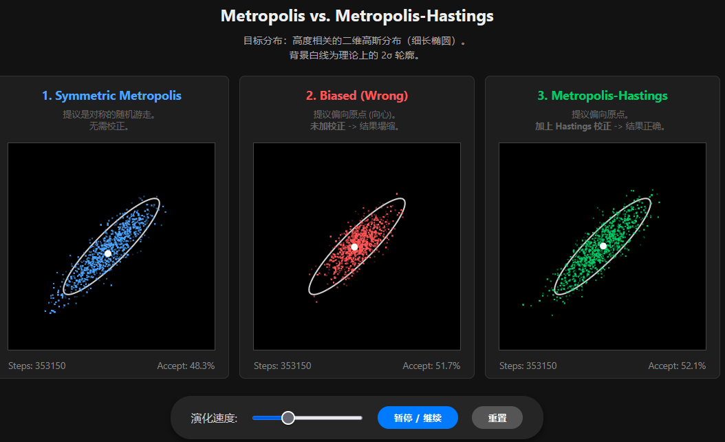
例子：二维高斯分布

假设我们要模拟的目标分布 $\pi(\mathbf{x})$ 是一个二维高斯分布，两个变量 $x_1, x_2$ 高度相关（形状像一个倾斜的细长椭圆）。

• 目标分布：$\mathbf{x} \sim \mathcal{N}(\mathbf{0}, \Sigma)$
• 协方差矩阵： \(\Sigma = \begin{pmatrix} 1 & 0.9 \\ 0.9 & 1 \end{pmatrix}\) （0.9 的相关性意味着两者倾向于同号）。
• 目标概率密度（忽略归一化常数）： \(\pi(\mathbf{x}) \propto \exp\left( -\frac{1}{2} \mathbf{x}^T \Sigma^{-1} \mathbf{x} \right)\)

设计不对称提议分布：向心漂移 (Centering Drift)

既然我们知道高斯分布的中心在 $(0,0)$，为了避免采样点跑得太远回不来，我们设计一个带有向心力的提议分布。

• 提议规则：下一步 $\mathbf{y}$ 不再以当前状态 $\mathbf{x}$ 为中心，而是以 $0.8 \mathbf{x}$ 为中心。这意味着每一步都有 20% 的趋势被拉回原点。 \(\mathbf{y} \sim \mathcal{N}(0.8\mathbf{x}, \sigma^2 \mathbf{I})\)

• 从外向里跳 ($x \to y$)：假设 $x=10$ (远)，提议中心是 $8$，如果 $y=8$ (近)，这很容易发生。
• 从里向外跳 ($y \to x$)：假设 $y=8$ (近)，提议中心是 $6.4$。如果要跳回 $x=10$ (远)，你需要逆着“向心力”跳，这非常困难。
• 不对称性：$g(x \to y) > g(y \to x)$（当 $y$ 比 $x$ 更靠近原点时）。

提议分布是高斯分布： \(g(\mathbf{y}|\mathbf{x}) \propto \exp\left( -\frac{\| \mathbf{y} - 0.8\mathbf{x} \|^2}{2\sigma^2} \right)\)

Hastings Ratio (校正因子)：

\[\frac{g(\mathbf{y} \to \mathbf{x})}{g(\mathbf{x} \to \mathbf{y})} = \frac{g(\mathbf{x}|\mathbf{y})}{g(\mathbf{y}|\mathbf{x})} = \frac{\exp\left( -\frac{\| \mathbf{x} - 0.8\mathbf{y} \|^2}{2\sigma^2} \right)}{\exp\left( -\frac{\| \mathbf{y} - 0.8\mathbf{x} \|^2}{2\sigma^2} \right)} = \exp\left( \frac{\| \mathbf{y} - 0.8\mathbf{x} \|^2 - \| \mathbf{x} - 0.8\mathbf{y} \|^2}{2\sigma^2} \right)\]

可视化代码

<!DOCTYPE html>
<html lang="zh">
<head>
    <meta charset="UTF-8">
    <title>Metropolis vs MH Comparison</title>
    <style>
        body {
            font-family: 'Segoe UI', sans-serif;
            background-color: #121212;
            color: #eee;
            display: flex;
            flex-direction: column;
            align-items: center;
            margin: 0;
            padding: 20px;
        }
        
        .title-group { text-align: center; margin-bottom: 20px; }
        h2 { margin: 0 0 10px 0; }
        p { color: #aaa; font-size: 0.9em; max-width: 900px; margin: 0 auto; line-height: 1.5; }

        .container {
            display: flex;
            gap: 15px;
            flex-wrap: wrap;
            justify-content: center;
        }
        
        .panel {
            background: #1e1e1e;
            padding: 10px;
            border-radius: 8px;
            text-align: center;
            border: 1px solid #333;
            width: 320px;
        }

        canvas {
            background: #000;
            border: 1px solid #444;
            margin-top: 10px;
        }

        h3 { margin: 5px 0; font-size: 1.1em; }
        .blue { color: #4da6ff; }
        .red { color: #ff5555; }
        .green { color: #00cc66; }

        .stats {
            margin-top: 8px;
            font-size: 0.85em;
            color: #888;
            display: flex;
            justify-content: space-between;
            padding: 0 10px;
        }

        .desc {
            font-size: 0.8em;
            color: #666;
            margin-top: 8px;
            min-height: 40px;
        }

        .controls {
            margin-top: 25px;
            background: #252525;
            padding: 15px 30px;
            border-radius: 30px;
            display: flex;
            gap: 20px;
            align-items: center;
            box-shadow: 0 4px 10px rgba(0,0,0,0.5);
        }

        button {
            padding: 8px 24px;
            background-color: #007bff;
            color: white;
            border: none;
            border-radius: 20px;
            cursor: pointer;
            font-weight: bold;
            transition: background 0.2s;
        }
        button:hover { background-color: #0056b3; }
        button.reset { background-color: #555; }
        button.reset:hover { background-color: #777; }
        
        input[type=range] { cursor: pointer; }
    </style>
</head>
<body>

    <div class="title-group">
        <h2>Metropolis vs. Metropolis-Hastings</h2>
        <p>目标分布：高度相关的二维高斯分布（细长椭圆）。<br>背景白线为理论上的 2σ 轮廓。</p>
    </div>

    <div class="container">
        <!-- 1. Symmetric Metropolis -->
        <div class="panel">
            <h3 class="blue">1. Symmetric Metropolis</h3>
            <div class="desc">提议是对称的随机游走。<br>无需校正。</div>
            <canvas id="canvasSym" width="300" height="300"></canvas>
            <div class="stats">
                <span>Steps: <span id="cntSym">0</span></span>
                <span>Accept: <span id="accSym">0%</span></span>
            </div>
        </div>

        <!-- 2. Biased Wrong -->
        <div class="panel">
            <h3 class="red">2. Biased (Wrong)</h3>
            <div class="desc">提议偏向原点 (向心)。<br><b>未加校正</b> -> 结果塌缩。</div>
            <canvas id="canvasWrong" width="300" height="300"></canvas>
            <div class="stats">
                <span>Steps: <span id="cntWrong">0</span></span>
                <span>Accept: <span id="accWrong">0%</span></span>
            </div>
        </div>

        <!-- 3. Biased Correct (MH) -->
        <div class="panel">
            <h3 class="green">3. Metropolis-Hastings</h3>
            <div class="desc">提议偏向原点。<br><b>加上 Hastings 校正</b> -> 结果正确。</div>
            <canvas id="canvasCorrect" width="300" height="300"></canvas>
            <div class="stats">
                <span>Steps: <span id="cntCorrect">0</span></span>
                <span>Accept: <span id="accCorrect">0%</span></span>
            </div>
        </div>
    </div>

    <div class="controls">
        <label style="color:#ccc">演化速度:</label>
        <input type="range" id="speedRange" min="1" max="100" value="10">
        <button onclick="toggleRun()" id="btnPause">暂停 / 继续</button>
        <button class="reset" onclick="resetSim()">重置</button>
    </div>

<script>

    // 目标分布：协方差 Sigma = [[1, 0.9], [0.9, 1]]
    const det = 1 - 0.9*0.9; 
    const invSigma = [
        [1/det, -0.9/det],
        [-0.9/det, 1/det]
    ];

    // 提议参数
    const ALPHA = 0.8;      // 向心系数 (0.8 表示下一步均值在 0.8*当前位置)
    const SIGMA_PROP = 0.6; // 提议步长的噪声
    
    // 对称游走的步长 (为了公平对比，稍作调整)
    const SIGMA_SYM = 0.6;  

    // 计算目标对数概率: -0.5 * x^T * Sigma^-1 * x
    function getLogTarget(x, y) {
        const val = x * (invSigma[0][0]*x + invSigma[0][1]*y) +
                    y * (invSigma[1][0]*x + invSigma[1][1]*y);
        return -0.5 * val;
    }

    // 计算提议对数概率 log q(to | from)
    // 对于对称游走，这个函数其实用不到 (结果会消掉)
    // 对于非对称，q(y|x) 是均值为 alpha*x 的高斯分布
    function getLogProposal(toX, toY, fromX, fromY) {
        const muX = ALPHA * fromX;
        const muY = ALPHA * fromY;
        const distSq = (toX - muX)**2 + (toY - muY)**2;
        return -0.5 * distSq / (SIGMA_PROP**2);
    }

    // 标准正态分布随机数生成器 (Box-Muller)
    function randn() {
        let u = 0, v = 0;
        while(u === 0) u = Math.random(); 
        while(v === 0) v = Math.random();
        return Math.sqrt( -2.0 * Math.log( u ) ) * Math.cos( 2.0 * Math.PI * v );
    }

    // --- 模拟类 ---
    class Simulation {
        constructor(canvasId, type, color) {
            this.canvas = document.getElementById(canvasId);
            this.ctx = this.canvas.getContext('2d');
            this.type = type; // 'symmetric', 'wrong', 'correct'
            this.color = color;
            
            this.history = [];
            this.reset();
            
            // 视图参数
            this.scale = 35; 
            this.cx = this.canvas.width / 2;
            this.cy = this.canvas.height / 2;
        }

        reset() {
            this.x = 3.5; // 初始点放远一点，观察收敛
            this.y = 3.5;
            this.history = [];
            this.total = 0;
            this.accepted = 0;
        }

        step() {
            this.total++;
            let nextX, nextY;
            let logCorrection = 0;

            // 1. 生成提议 (Proposal)
            if (this.type === 'symmetric') {
                // 对称游走: next = current + noise
                nextX = this.x + randn() * SIGMA_SYM;
                nextY = this.y + randn() * SIGMA_SYM;
                // 对称提议，校正因子 log(1) = 0
                logCorrection = 0;
            } else {
                // 非对称游走: next = 0.8 * current + noise
                const muX = ALPHA * this.x;
                const muY = ALPHA * this.y;
                nextX = muX + randn() * SIGMA_PROP;
                nextY = muY + randn() * SIGMA_PROP;
                
                if (this.type === 'correct') {
                    // Hastings Correction
                    // log [ q(old|new) / q(new|old) ]
                    const logQ_back = getLogProposal(this.x, this.y, nextX, nextY);
                    const logQ_fwd  = getLogProposal(nextX, nextY, this.x, this.y);
                    logCorrection = logQ_back - logQ_fwd;
                } else {
                    // 'wrong' 类型，忽略校正
                    logCorrection = 0;
                }
            }

            // 2. 计算接受率
            const logTargetDiff = getLogTarget(nextX, nextY) - getLogTarget(this.x, this.y);
            const logAlpha = logTargetDiff + logCorrection;

            // 3. 接受/拒绝
            if (Math.log(Math.random()) < logAlpha) {
                this.x = nextX;
                this.y = nextY;
                this.accepted++;
            }

            // 存入历史 (限制长度以保证性能)
            this.history.push({x: this.x, y: this.y});
            if (this.history.length > 2000) this.history.shift();
        }

        draw() {
            // 清屏
            this.ctx.fillStyle = "#000";
            this.ctx.fillRect(0, 0, this.canvas.width, this.canvas.height);

            // 画理论椭圆 (2 Sigma)
            // 协方差矩阵特征值 approx 1.9, 0.1
            // 2 Sigma 长轴 ~ 2*sqrt(1.9) ~ 2.75, 短轴 ~ 2*sqrt(0.1) ~ 0.63
            // 旋转 45度
            this.ctx.strokeStyle = "rgba(255, 255, 255, 0.85)";
            this.ctx.lineWidth = 2;
            this.ctx.beginPath();
            for (let t = 0; t <= Math.PI * 2; t += 0.1) {
                const a = 2.75; const b = 0.63;
                const _x = a * Math.cos(t);
                const _y = b * Math.sin(t);
                // 旋转变换
                const rX = _x * 0.707 - _y * 0.707;
                const rY = _x * 0.707 + _y * 0.707;
                this.ctx.lineTo(this.cx + rX * this.scale, this.cy - rY * this.scale);
            }
            this.ctx.closePath();
            this.ctx.stroke();

            // 画点
            this.ctx.fillStyle = this.color;
            // 为了视觉效果，旧点暗一些，新点亮一些
            for (let i = 0; i < this.history.length; i++) {
                const p = this.history[i];
                const alpha = 0.2 + 0.8 * (i / this.history.length); // 透明度渐变
                this.ctx.globalAlpha = alpha;
                this.ctx.fillRect(this.cx + p.x * this.scale - 1, this.cy - p.y * this.scale - 1, 2, 2);
            }
            this.ctx.globalAlpha = 1.0;

            // 画当前位置大点
            this.ctx.beginPath();
            this.ctx.arc(this.cx + this.x * this.scale, this.cy - this.y * this.scale, 5, 0, Math.PI*2);
            this.ctx.fillStyle = "#fff";
            this.ctx.fill();
        }
    }

    // --- 主控逻辑 ---
    const simSym = new Simulation('canvasSym', 'symmetric', '#4da6ff');
    const simWrong = new Simulation('canvasWrong', 'wrong', '#ff5555');
    const simCorrect = new Simulation('canvasCorrect', 'correct', '#00cc66');
    
    let isRunning = true;
    let speed = 10;
    
    // UI 引用
    const uis = [
        {sim: simSym, cnt: 'cntSym', acc: 'accSym'},
        {sim: simWrong, cnt: 'cntWrong', acc: 'accWrong'},
        {sim: simCorrect, cnt: 'cntCorrect', acc: 'accCorrect'}
    ];

    function loop() {
        if (isRunning) {
            for (let k = 0; k < speed; k++) {
                simSym.step();
                simWrong.step();
                simCorrect.step();
            }
            
            uis.forEach(u => {
                u.sim.draw();
                document.getElementById(u.cnt).innerText = u.sim.total;
                document.getElementById(u.acc).innerText = (u.sim.accepted / u.sim.total * 100).toFixed(1) + "%";
            });
        }
        requestAnimationFrame(loop);
    }

    function toggleRun() {
        isRunning = !isRunning;
    }

    function resetSim() {
        simSym.reset();
        simWrong.reset();
        simCorrect.reset();
        uis.forEach(u => u.sim.draw());
    }

    document.getElementById('speedRange').oninput = function() {
        speed = parseInt(this.value);
    };

    loop();

</script>
</body>
</html>